Week 1 - Preliminaries
Monday, September 14, 2020
“To know your future, you must know your past” ― George Santayana
Introduction
Before taking a deep dive into election result predictions, I thought it would be of great interest to investigate some of the parallel universes, or contributing factors if you would like, of election night results. This week, we look at swing states and how we can identify those based on historical trends, and investigate the effect of turnout to the popular vote results.
Uncovering Swing States
Using the historical approach
We begin by looking at the differences between the popular vote percentage that Democrats received in a given election and the popular vote percentage that the party received in the previous election cycle. We use the two-party (Republican and Democrat) popular vote sum to calculate the percentages, as none of the independent or third-party candidates have secured any electoral votes in the period 1984-2016 we are considering (Dave Leip’s Atlas of U.S. Presidential Elections). We will spend some time exploring the impact of the third-party vote (i.e., in the 2000 presidential election in Florida) in a future blog post.
To calculate the swing percentage we use the following formula:
, where
and
are the popular vote percentages that the Democratic and Republican candidate received in year i respectively, and
and
are the popular vote percentages that the Democratic and Republican candidate received in previous election cycle respectively.
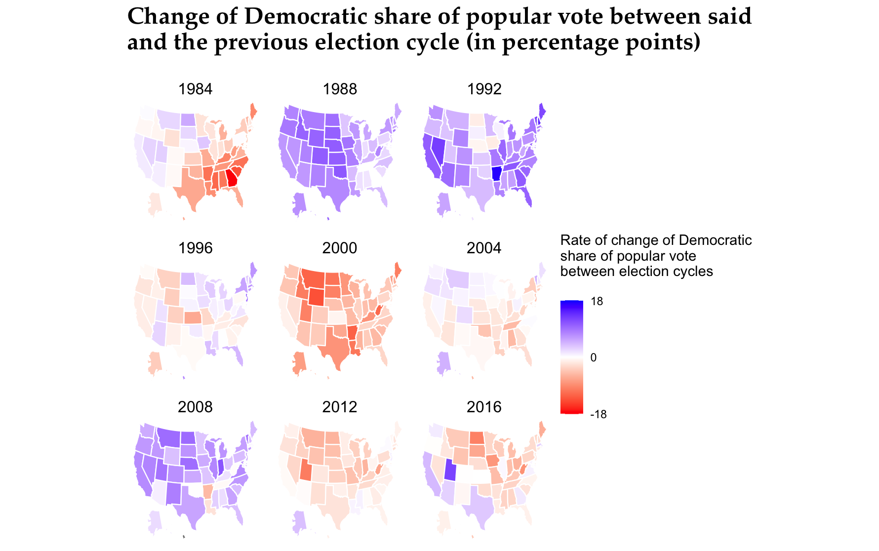
Working with the data from the popular vote results for both parties on the elections of 1980 to 2016, we generated the following map:
 Please note that because of the nature of the formula we use to calculate the change in percentage of the popular vote, we cannot create a map for the year 1980, but use it to create the map for the year 1984.
In the map, a deeper blue color of a state denotes that the Democratic party saw substantial increases in the percentage of the popular vote they secured against their Republican contenders compared to the previous election. On the other hand, a deep red color points to a strong Republican resurgence in the state’s popular vote results compared to the percentage scored four years before.
One of the first things we can point out in the popular vote distribution is the sudden surge of the Democratic share of the popular vote in almost all states around the United States. This is quite understandable based on the 2008 “Obama effect,” who secured 52.93% of the popular vote and a landslide 67.84% (365/538) of the electoral votes. We observe similar results when a “change of guard” happens between the two main competing parties. An interesting exception, however, is the 1988, when George H. W. Bush was elected: the whole country turned blue, as a result of the stark decline of the electoral vote share (79.18% vs. 97.58%) and popular vote share (53.37% vs. 58.77%) that Bush secured compared to the lanslide victory of Ronald Reagan 4 years before.
In terms of the current political climate, we take a look at the times the rate of change of the Democratic share of popular votes in a state changed sign (Democratic share of popular votes started decreasing after increasing, or started increasing after declining in the previous election). We present the results of this analysis in the following table, and highlight specific states we are going to discuss in greater detail in boldface.
| State | 2016 Change | 2012 Change | 2008 Change | Times change rate sign flipped |
|---|---|---|---|---|
| Alabama | 2.01 | -0.33 | -3.16 | 1 |
| Alaska | 2.16 | 3.75 | -1.07 | 1 |
| Arizona | 0.96 | -0.30 | 2.72 | 2 |
| Arkansas | -5.24 | -1.98 | -2.13 | 0 |
| California | 7.24 | -0.41 | 4.26 | 2 |
| Colorado | 6.92 | -1.80 | -0.06 | 1 |
| Connecticut | 6.04 | -2.55 | -1.63 | 1 |
| Delaware | 8.81 | -3.19 | -3.45 | 1 |
| District of Columbia | 2.88 | -0.81 | 3.11 | 2 |
| Florida | 3.94 | -0.98 | -1.06 | 1 |
| Georgia | 5.73 | -1.33 | 1.30 | 2 |
| Hawaii | 18.59 | -1.29 | -4.26 | 1 |
| Idaho | 6.30 | -3.40 | -1.89 | 1 |
| Illinois | 7.53 | -4.16 | 0.44 | 2 |
| Indiana | 10.95 | -5.72 | -4.92 | 1 |
| Iowa | 5.19 | -1.89 | -8.02 | 1 |
| Kansas | 5.25 | -3.50 | 0.00 | 2 |
| Kentucky | 1.77 | -3.31 | -4.13 | 1 |
| Louisiana | -2.13 | 0.71 | -1.42 | 2 |
| Maine | 4.25 | -0.97 | -6.26 | 1 |
| Maryland | 6.36 | 0.39 | 0.69 | 0 |
| Massachusetts | 0.45 | -1.41 | 2.87 | 2 |
| Michigan | 6.65 | -3.57 | -4.92 | 1 |
| Minnesota | 3.47 | -1.29 | -3.11 | 1 |
| Mississippi | 2.86 | 0.84 | -3.29 | 1 |
| Missouri | 3.55 | -4.71 | -5.04 | 1 |
| Montana | 9.33 | -5.86 | -4.08 | 1 |
| Nebraska | 9.24 | -3.52 | -2.42 | 1 |
| Nevada | 7.70 | -2.98 | -2.11 | 1 |
| New Hampshire | 4.18 | -2.03 | -2.64 | 1 |
| New Jersey | 4.49 | 1.09 | -1.67 | 1 |
| New Mexico | 8.07 | -2.37 | -0.64 | 1 |
| New York | 5.93 | 0.28 | -2.63 | 1 |
| North Carolina | 6.41 | -1.20 | -0.87 | 1 |
| North Dakota | 9.50 | -5.70 | -9.70 | 1 |
| Ohio | 3.39 | -0.82 | -5.78 | 1 |
| Oklahoma | -0.07 | -1.13 | -2.53 | 0 |
| Oregon | 6.31 | -2.14 | -0.12 | 1 |
| Pennsylvania | 3.97 | -2.50 | -3.11 | 1 |
| Rhode Island | 3.62 | -0.18 | -5.71 | 1 |
| South Carolina | 4.09 | -0.76 | -2.15 | 1 |
| South Dakota | 6.62 | -4.92 | -6.75 | 1 |
| Tennessee | -0.45 | -2.72 | -3.27 | 0 |
| Texas | 5.57 | -2.07 | 3.29 | 2 |
| Utah | 8.82 | -10.10 | 12.24 | 2 |
| Vermont | 8.60 | -0.65 | -3.06 | 1 |
| Virginia | 7.32 | -1.22 | 0.86 | 2 |
| Washington | 5.11 | -1.12 | 1.16 | 2 |
| West Virginia | -0.19 | -7.00 | -8.49 | 0 |
| Wisconsin | 6.86 | -3.59 | -3.87 | 1 |
| Wyoming | 3.75 | -4.60 | -4.54 | 1 |
We can define swing states in many different ways. One definition could be a state in which the rate of change in the Democratic share of the popular vote between elections changes signs in every pair of election cycles (e.g., Georgia, Arizona, Texas, Utah). The rationale behind this definition is that abrupt changes in the Democratic share of the popular vote between elections are usually caused by ideological shifts of undecided voters that swing the popular votes, the state’s electoral college votes, and potentially the whole election.
On the other hand, we could define states as swing states when the sum of the rates of change over the last three pairs of election cycles is close to zero (e.g. Florida, Maine, Michigan, New Hampshire, North Carolina, Pennsylvania, South Carolina, Wisconsin). This definition takes into account the general historical development of election results in each state. A sum value close to zero shows that even though there might be some changes in the share of the popular vote between elections, the overall change in the share of the popular vote is quite stable. This creates a trend of a supposed equilibrium that could influence the results of future elections. In either case, our analysis identifies the “Big Four” states correctly, which might ultimately decide the outcome of the election WSJ, 2020.
Does turnout affect the results?
Let’s continue with the analysis of turnout and the share of popular vote results between the two main parties. Using the data from Dave Leip’s Atlas of U.S. Presidential Elections, we compiled a CSV file for the election turnout statistics for elections beginning in 1942. We created the following plot to examine the relationship between those two measures:
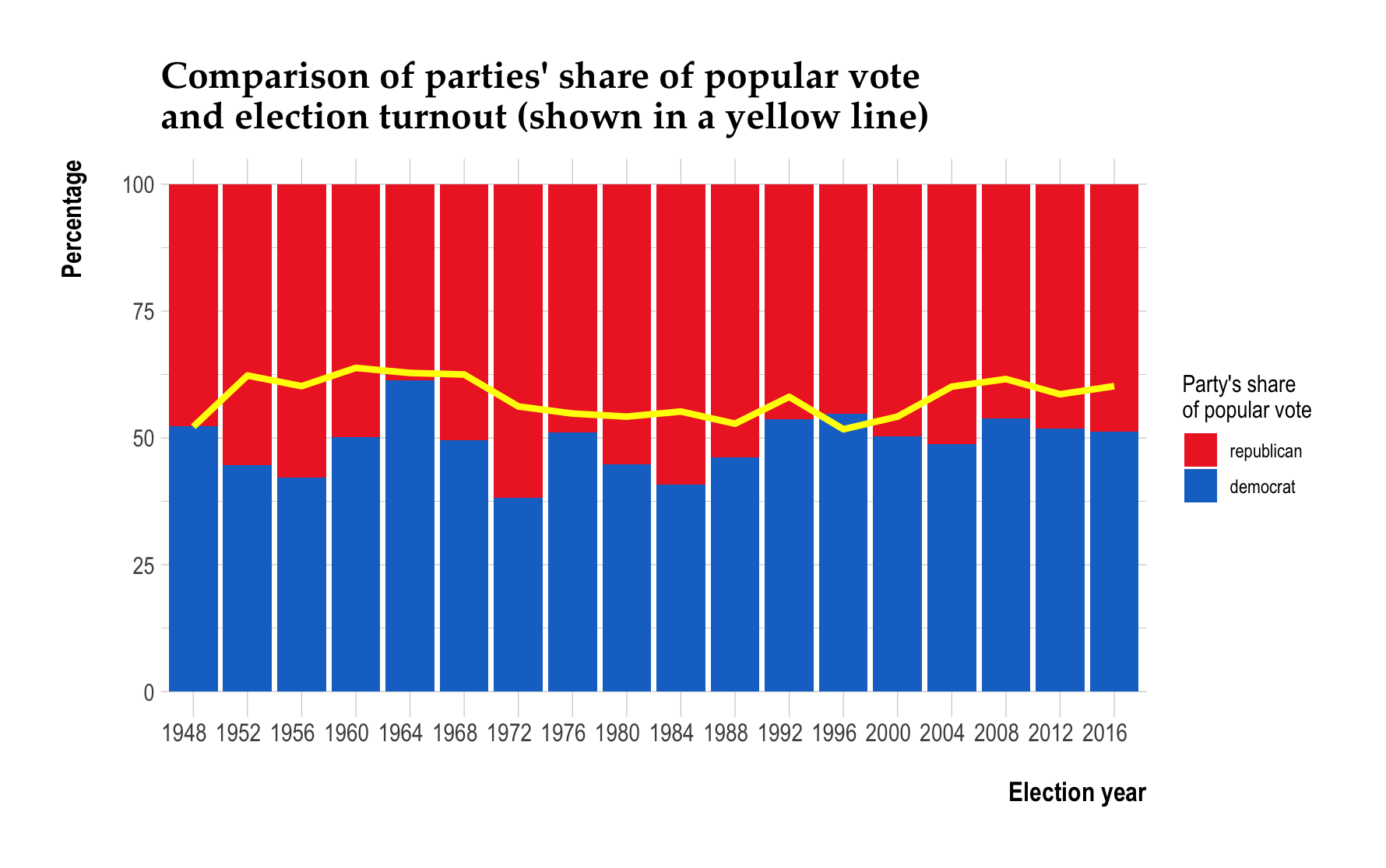 We see that, especially in the last few decades, a rise in turnout generally gives Democrats an advantage in the popular vote, with 2008 being a prime example of this trend. On the other hand, we see that in election years like 1956, 1972, and 1984, when voter turnout is considerably low, the Republican popular vote share soars. It would be particularly exciting to research the effect of youth’s turnout rates in election results, as the turnout of older generations usually is stable (Binstock, 2000).
Onwards
As we are looking forward to another week and coming closer to election day, we will start devising and implementing our own election prediction models while critically reviewing other researchers and political scientists’ models.