Final Election Prediction - It all comes down to this
Sunday, November 1, 2020
“pluralitas non est ponenda sine necessitate: plurality should not be posited without necessity.” ~ Scholastic philosopher William of Ockham
Introduction
The election is right around the corner, and we are ready to make our final prediction for the 2020 General Presidential Election. This time we use a three-step model to grapple with the idiosyncrasies of each state. Using our model, we determine the popular vote winner in each state, along with the winner of the Electoral College vote.
Model Ideation and Walkthrough
Our model relies on three different parts:
(a) an initial prediction of candidates’ popular vote share based on a weighted model of poll ranking and a decay-over-time effect for each poll’s impact on the final result,
(b) a probabilistic model that predicts the popular vote share using turnout estimates based on the age of the population, the popularity of mail-in and early voting, and the COVID-19 spread in the state, and
(c) an ensemble of the two predictions to correct the probabilistic model’s uncertainty and tie everything back together to produce the final result.
Part I: Weighted Poll Results
As we saw in our Week 3 blog, FiveThirtyEight provides poll ratings based on each poll’s Predictive Plus-Minus rating, which aims to address the variation between methodological standards score and accuracy differences between each poll and includes a “herding penalty” for pollsters with low methodology ratings. As we get much closer to Election Day and more independent (i.e., unaffiliated) or undecided voters make up their mind, polls become even more accurate in predicting the actual popular vote share. Therefore, we have decided to use the weighted model based on poll ratings to essentially “sort through” all 50 states and determine which ones we should denote as “battleground states” that require further analysis to determine the actual winner.
As we saw in our Week 3 blog, FiveThirtyEight provides poll ratings based on each poll’s Predictive Plus-Minus rating, which aims to address the variation between methodological standards score and accuracy differences between each poll and includes a “herding penalty” for pollsters with low methodology ratings. As we get much closer to Election Day and more independent (i.e., unaffiliated) or undecided voters make up their mind, polls become even more accurate in predicting the actual popular vote share. Therefore, we have decided to use the weighted model based on poll ratings to essentially “sort through” all 50 states and determine which ones we should denote as “battleground states” that require further analysis to determine the actual winner.
Our model uses the poll weighting method described below. For each of the poll ratings, we use the following scoring function, where x represents each one of the poll results:
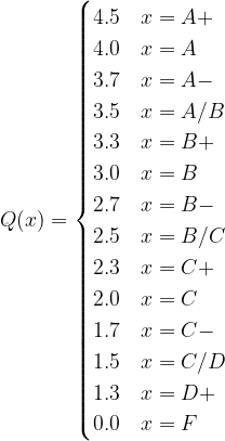
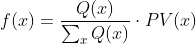
We chose the specific grading scheme, resembling that of a course grading scale, because as we saw in Week 3, and shown in the graph below, where we obtained by analyzing the distribution of letter poll ratings that FiveThirtyEight provides based on each poll’s Predictive Plus-Minus rating, there is a large number of polls that are rated B/C, and a few rated higher or lower. Therefore, a 2.5/4 score for a B/C-rated poll constitutes an average score, meaning that our model “awards” polls of higher quality and almost disregards low-scoring polls, as expected. To normalize all election poll results and calculate the “contribution” of each result to the final calculated popular vote share of a candidate, we divide each score over the sum of all poll scores and then multiply it with the actual poll-predicted state popular vote share:
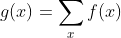
Finally, the state popular vote share calculated for a specific candidate is:
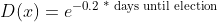
However, we also wanted to control for the time since the poll was conducted, as the decay-over-time model we incorporate states that because of the constant changes in the presidential battlefield, polls lose their predictive power over time. We decided to exclude polls that were concluded at least 42 days before the election, as that polling performance became increasingly irrelevant to current events. For instance, Arizona voters surveyed before Sunday, September 22nd, would not have been informed about the President contracting COVID-19, watched any presidential debates, or read about the President’s $750 tax payment. Lastly, it is understandable to assume that many independent and undecided voters are less likely to make up their minds before the presidential debates, so polling after that period becomes increasingly more relevant. We use the model of exponential decay to model this relationship. Testing out many different values for λ, and wanting to give some significant consideration to the polls of the last week before the election, we obtain the following poll weighting model,
To normalize all election poll results and calculate the “contribution” of each result to the final calculated popular vote share of a candidate, we divide each time decay poll value over the sum of all time decay poll values and then multiply it with the actual poll-predicted state popular vote share:
Finally, the state popular vote share calculated for a specific candidate is:
Then, we needed to weigh each result to determine our final predicted popular vote share result. For this, we decided to trust the accuracy of the polls close to Election Day, and weighted the poll ranking model a little more compared to the decay model (0.6 vs 0.4), to get the following final model for the state popular vote share calculated for a specific candidate:

At this time, we identified the following 7 “battleground” states that had a candidate popular vote margin less than six percentage points: Arizona, Florida, Georgia, Iowa, Nevada, North Carolina, Ohio, Pennsylvania, and Texas. We chose the six percentage point benchmark, as we wanted to limit the number of “battleground” states, but also did not want to rely entirely on the polls model where the margin of victory was quite slim. The following table presents the popular vote share predictions and the absolute difference between the two candidates:
| State | Democratic Popular Vote Share | Republican Popular Vote Share | Absolute Difference (Win Margin) |
|---|---|---|---|
| Arizona | 49.53 | 45.60 | 3.93 |
| Florida | 48.89 | 46.77 | 2.13 |
| Georgia | 48.97 | 46.88 | 2.09 |
| Iowa | 47.42 | 47.96 | 0.54 |
| Nevada | 50.29 | 45.66 | 4.63 |
| North Carolina | 49.35 | 46.52 | 2.84 |
| Ohio | 47.16 | 48.65 | 1.49 |
| Pennsylvania | 50.78 | 44.90 | 5.88 |
| Texas | 47.15 | 48.67 | 1.52 |
Part II: Turnout Prediction and Binomial Processes
To determine our final prediction for those seven battleground states, we turn to the turnout prediction and probabilistic models we implemented in the last few weeks.
The vote total for any particular candidate in the presidential election has a fixed set of possible values: 0 − VEP, where VEP is the voter eligible population for the presidential election in question. Let’s say we’re interested in the popular vote total for the Democratic nominee in some state s. Thus, the election outcome for Democrats in state s is some draw of voters from the voter-eligible population (VEPs) turning out to vote Democrat. We call this process of draws from a population (often called successes from a number of trials) a binomial process.
The core probabilistic phenomena driving a binomial process is whether or not a single voter, denoted by i, will turn out and vote for the party in question. Let’s call this individual voter probability in state s. The question we can ask is: what, then, is the probability of n voters voting for the Democratic presidential nominee in this state? It turns out that this question can be answered by setting up a distribution that follows the Binomial distribution.
To improve our probabilistic model, and account for any model outliers, instead of a calculating the probability for a single Democratic voter showing up to the polls and voting for the Democratic presidential nominee, or the single expected number of Democratic voters from the population, we predict a distribution of Democratic voter draws from the respective binomial process on that population.
We simulate draws from 100,000 repeated Binomial process with a population of size VEP and a draw probability of predicted draw probabilities for Democrats and Republicans based on the binomial distribution model, derived from previous election cycles. Finally, we are simulating a distribution of election results, specifically calculating Biden’s win or loss (if negative) margin in each state, and then attributing the electoral votes of each state to the winner of that state. Note: absent specific polling results of each of the electoral districts in Maine and Nebraska, we assume that the general state vote will reflect on the distribution of those electoral votes and follow the usual “winner takes all” electoral college vote distribution model.
To make our model more accurate, we expand our probabilistic model by incorporating the factor of turnout. Rather than fixing each state’s maximum number of Binomial draws to the state’s VEP, we draw a random number from a distribution constructed using VEP and our guess on the effect of COVID and vote-by-mail). To do so, we employ the following statistics:
- percentage of people that are older than 65 years old: we expect that this age group is more prone to COVID-19, but less accustomed to vote by mail. Therefore, they more likely to vote in person or be hesitant to turn out to vote. The model attaches the weight
-0.2account for a significant, but not overwhelming effect, as we assume that a considerable number of elderly will still show up at the polls. - number of COVID-19 cases per 100 thousand state residents: we assume that a high COVID-19 case number will deter voters from voting in-person, especially when they are not accustomed to early or absentee voting. We give a coefficient of
-0.3, as we expect this to affect the whole voting-eligible population and not just older voters. Moreover, we expect that in the extreme case of 200 COVID-19 cases per 100 thousand state residents, the state will be on high alert, and the voting will be significantly affected, so we divide by the case number by 200. - percentage of the VEP that has already voted early (either in-person or by absentee ballot): shows us which states are on track to become gross mail-in or early voting states. In that case, we assume that people are more accustomed to the process, or COVID-19 has urged more people to vote early. The model attributes the coefficient of
0.4, as we expect early voting to be an efficient way for voting this year, signaled by the monumental early voting turnout rates, and we add the case rate described above to account for the increase in early voting numbers by the increase in COVID-19 positivity rates. The final turnout model is described below:
turnout = turnout_2016 * (1 - 0.2 * df$older_than_65 + 0.4 * (total_early_rates + 7day_COVID-19_cases_100K/200)- 0.3 * 7day_COVID-19_cases_100K/200)
For a final fix of accuracy, we set the standard deviation of the probabilistic general VEP prediction to 0.02 and the standard deviation of the probabilistic voter turnout prediction to 0.01, as we assume that our uncertainty for the turnout calculations will be higher than the uncertainty of polls so close to Election Day.
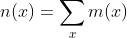
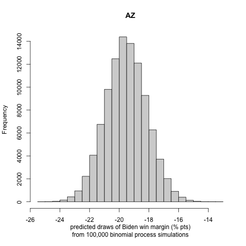
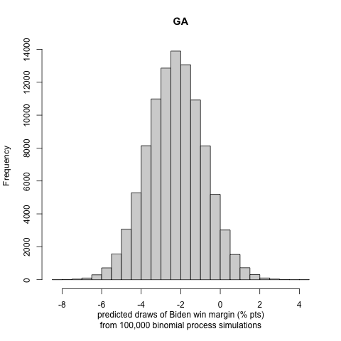
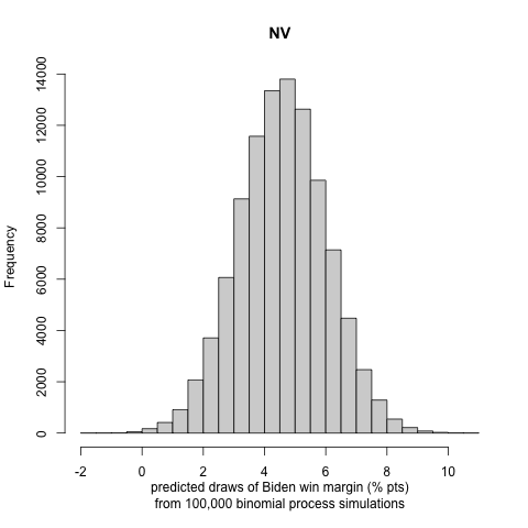
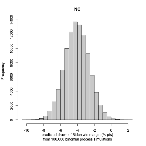
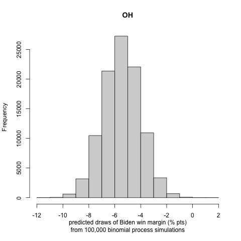
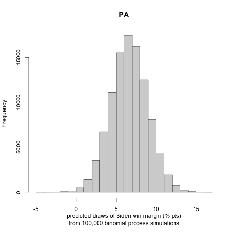
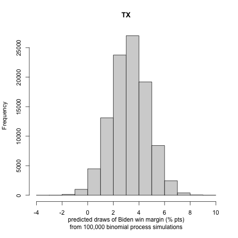
We generate histograms of Biden’s win or loss (if negative) margin in each state. We report the following exciting and note-worthy results for the nine battleground states to let the reader understand the incentive to follow the approach in part III:
 |
 |
 |
|---|---|---|
 |
 |
 |
 |
 |
 |
Part III: Model Correction Using Ensamble
As we see in the popular vote winning margins graphs above, in many of these battleground states, which are supposed to be too close to call, the winning margins are double digits, with the popular vote winning margins being highly polarized or having a sizeable possible value and uncertainty interval. To correct for that, we create an ensemble model combining the two models: the poll ranking (denoted by rank(x)) and the probabilistic and turnout model (denoted by prob(x)) to reach the final model (denoted by final(x)) for each battleground state x:

We spent a long time trying to find the best coefficients for w1 and w2. However, a guiding principle was that we should give high importance to the well-established model of poll rankings and then incorporate Election Day’s unpredictability using the second model. Therefore, we decided on the following two sets of coefficients: w1 = 0.8, w2=0.2 and w1 = 0.7, w2=0.3 that achieve that effect.
Uncertainty Around Prediction and Reflection
Using the two models (let’s call them conservative and explorational, as they give different weight to the poll averages), we calculate the results for each of the nine battleground states. We get the following map for the conservative model:
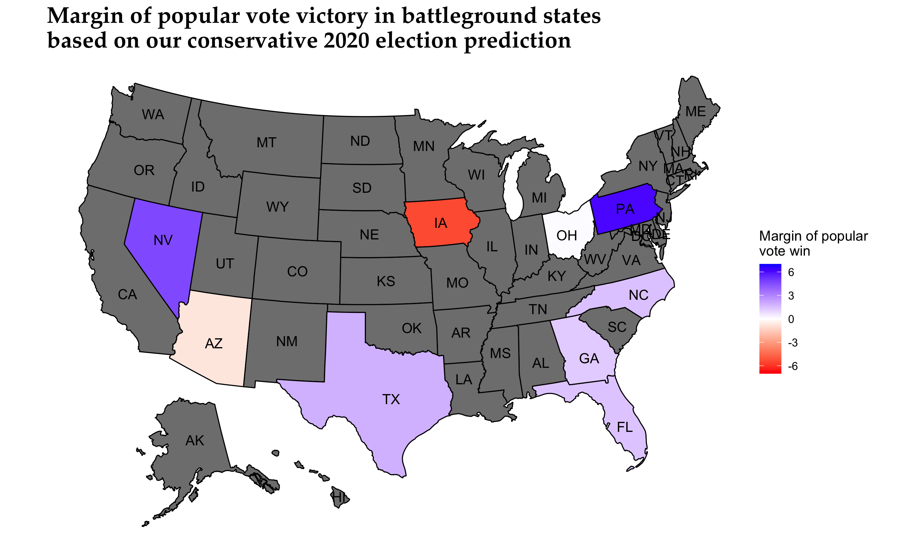
We can see that the closest race is that of Ohio, with Former Vice President Biden winning the state with a 0.10% mean voting margin (the prediction interval in the graph above is about 12 percentage points). However, mind the short legend color scheme when considering how polarized the other winning margins are. When we test for the explorational model, we get the following map for the nine battleground states:
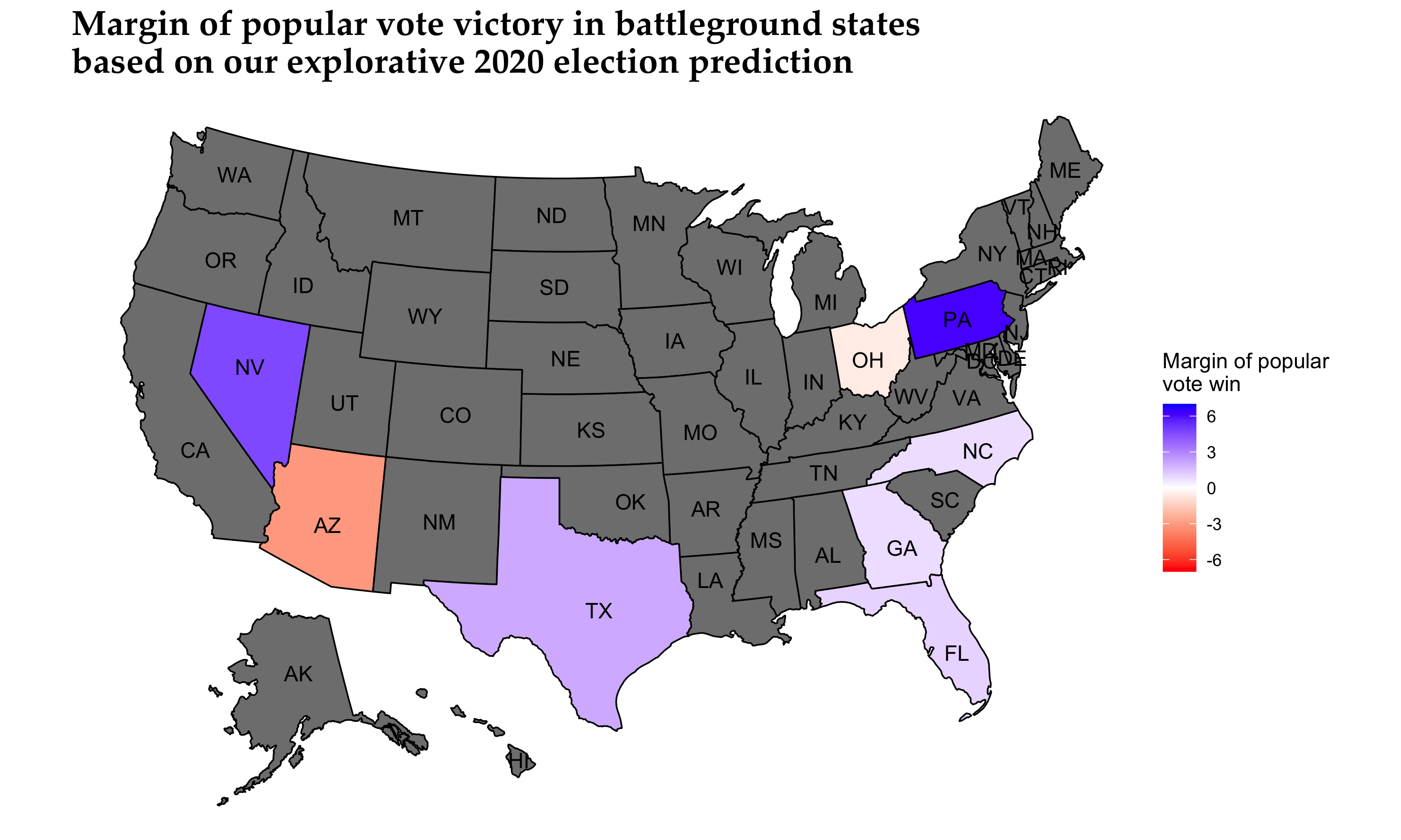
We observe that most states remain on the same party’s winning list, while some states increase their winning margins. However, Ohio is now won by President Trump with a 0.60% mean voting margin (as mentioned before, the prediction interval in the graph above is about 12 percentage points).
It is hard to define a national popular vote share and its respective uncertainty interval, based on our state results, and we believe that a national popular vote share is misleading for many audiences in determining the winner of the election. Finally, we chose not to integrate the successful 3rd Quarter GDP model that we developed in Week 2 even though the American economy has significantly improved in the last few months. Still, we do not believe that the economy is one of the most important issues that concern voters per se, as shown in recent opinion polls, and the economy was not one of the main standalone topics in the presidential debates. We also took into account Occam’s razor to decide that another variable would add more noise and complexity to our model and create more harm than good.
Our probabilistic model that incorporates the turnout prediction does not allow for in-sample or out-of-sample validation, as we do not have previous presidential elections affected by COVID-19 to fit and compare to. Some future studies on the effects of turnout by COVID-19 in the primaries to perform model validation might be an exciting and rewarding project. We see that there are large uncertainty intervals in the winning margin distributions of the binomial trials. Nonetheless, we observe that, in most cases, the most significant portion of the distribution curve lies on one candidate’s side, making us less concerned about the possibility of a highly inaccurate result. This conclusion is also justified by many states’ curves being strongly polarized (i.e., lying in a high winning margin region).
Prediction Results
This is the moment we have been waiting for. We have the following two U.S. winning margin graphs based on our conservative and explorative models:
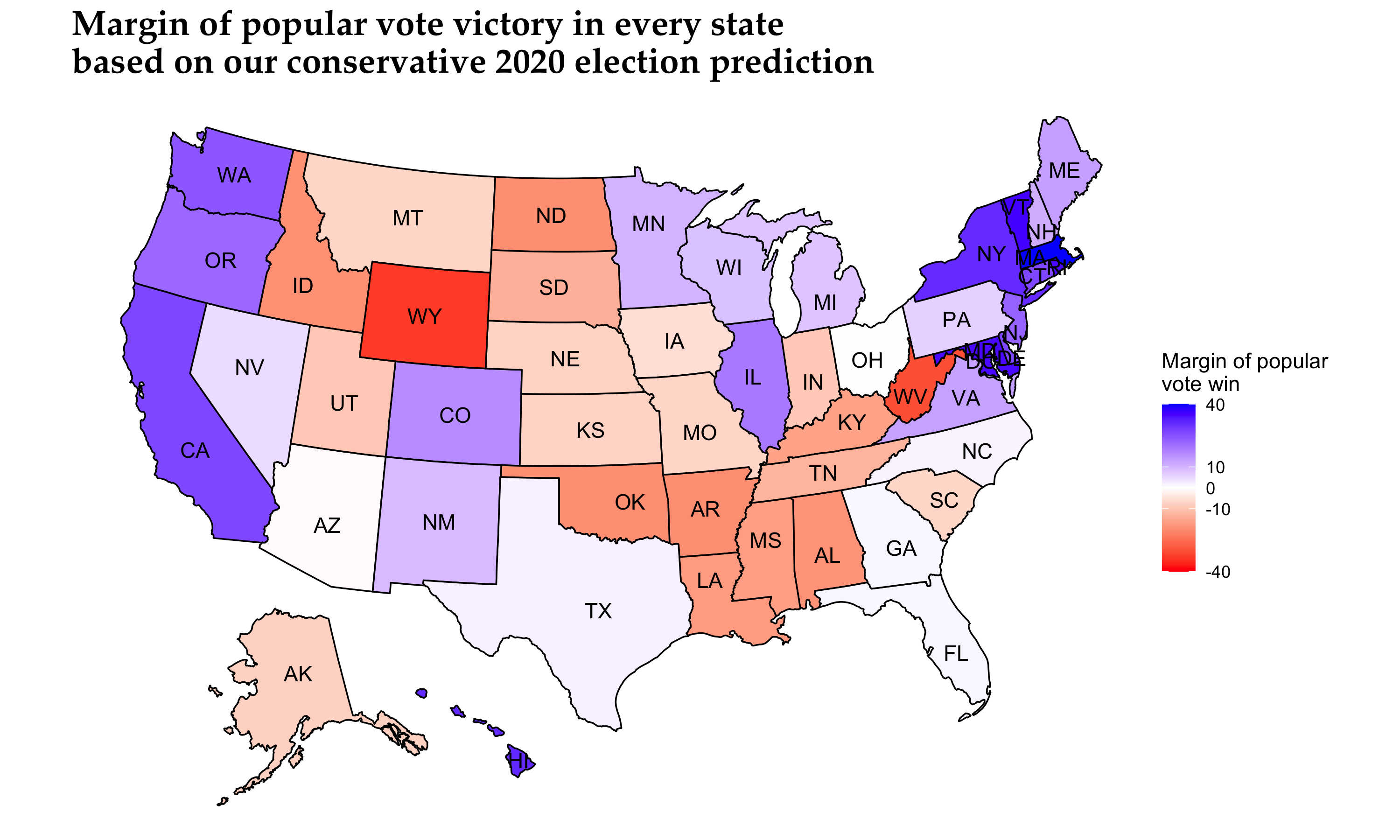
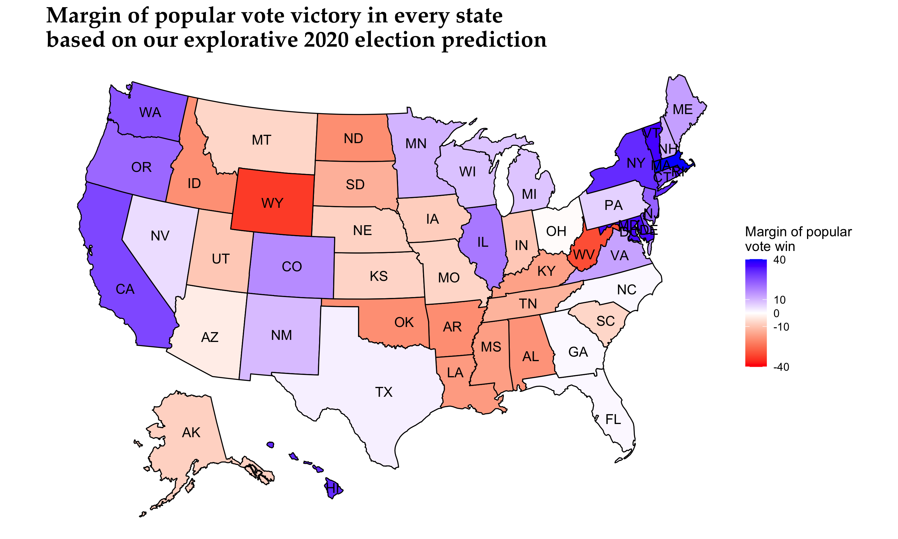
For simplicity and clarity, we report the following Electoral College vote counts based on our two models:
| Model | Democratic Electoral College vote count | Republican Electoral College vote count |
|---|---|---|
| Conservative | 311 | 226 |
| Explorative | 308 | 229 |
In the general sense, our model predicts the electoral vote share result quite close to FiveThirtyEight’s Biden win prediction, a little more conservatively nonetheless (Biden: 348 electoral votes, Trump: 190 electoral votes).
Look under the hood
Feel free to test out our model using the R code and datasets, conveniently uploaded in a ZIP file and our R Script here.
Onwards
As we are finally coming closer to election day, we will evaluate the election prediction model while critically reviewing other researchers and political scientists’ models.